Separate methods are required to analyze durations mainly for three reasons: (i) durations generally follow a highly skewed distribution – some subjects tend to have large and very large duration whereas most will have relatively short; (ii) study of duration requires follow-up and some subjects tend to be lost – they move away, refuse to cooperate further, do not report for follow-up, etc; and (iii) any follow-up is necessarily for a specified period and by the time you terminate the study, some subjects may not have reached to the end-point of interest – they are still alive, still feeding the child, still not recovered, etc. In the last two cases, the duration is incomplete – you only know that the duration is at least that much but do not know exactly how much. For example, if you are observing infants for duration of breast feeding and decide to follow-up 80 children for 6 months, it is possible that 4 are lost midway to follow-up (drop outs) and another 12 still on breast at the end of six-month period. Such values are called censored values. Because of censoring, statistics such as mean can not be calculated in a standard manner – neither the standard deviation. Thus a separate method is required. A measure such as person-months is also not applicable in this case; first, because of its inherent deficiency of considering first month as important as say sixth month and second, because censored values are treated same way as complete values.

Rather than the mean, the median survival duration is generally used in survival analysis. The other parameters of interest could be the entire ‘survival’ curve that is based on percentage of people existing at various time points, survival rate at specific time such as what percentage of children were on breastfeed at 4 months, and the duration by which, say 90%, reach the end-point—such as out of 80 children, at what time only 8 are left on breast milk, or at what time point, the survival is 10%. The methods of survival analysis adequately provide for censored values that the usual methods fail to do. However these methods depend on the type of censoring in the data as discussed in a short while. Survival analysis is also used for estimating hazards as explained later.

Besides modeling the survival pattern over a period of time, the other objectives of survival analysis are (i) to investigate factors that influence the duration of survival, (ii) to compare two or more modalities for survival pattern, and (iii) to estimate the future survival of individuals or groups with specified features. Among many methods available for survival analysis, in this communication we discuss only the more commonly used methods, namely, the life-table, Kaplan-Meier, log-rank and Cox model. This might help those who have duration data but are not comfortable in using survival analysis methods due to intricacies. We are trying to present them in simple language for our medical fraternity to increase awareness and to demystify the methods. All the survival methods we discuss are nonparametric or semiparametric and suit most types of duration. There might be isolated examples where parametric models may be more accurate(7).

Survival pattern helps patients and physicians to decide which treatment or health strategy to prefer and when. For example, short term survival may be better (in terms of percentage) with one regimen and long-term survival with another. For some conditions such as peritonitis, deaths are rapid and the survival curve shows quick decline. For others, such as kidney diseases, it may remain steady. The survival patterns are lessons to health care providers and seekers about what to expect in specific group of cases. The actual experience in individuals can vary but not too much if the survival curves are valid and reliable. Validity depends on correct recording of duration based on sharply defined starting and end-points on representative sample of subjects, and reliability depends on reasonable sample size.

Breastfeeding practically for all children starts from the day of birth but consider duration of childhood disease that can start at any age. When you start the study, if the child was already suffering, the exact starting time of the disease may not be known. This is called left censoring. Right censoring is the one discussed earlier where the ending time is not known. This is very common. Both these censoring are illustrated in Fig 1, including the completed observations and incomplete values. Hollow squares show right censoring.

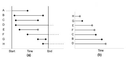Fig. 1 (a) Left and right censoring, (b) subjects ordered by available durations excluding person A with left censoring.

Third type of censoring occurs when you are asking patients to report at monthly intervals or conducting home visits, say, at every 3 months, to assess the status. In this case, only the interval will be known but not the exact duration. This is called grouped-interval censored data. In this setting also, right or left censoring can occur.

Left censoring is rare in duration studies and inadvisable as it complicates the analysis. We exclude this from our consideration in this communication. In addition, the general methods of survival analysis require the following:

An editorial(8) has discussed how biased results may have been obtained in survival analysis that does not check these requirements. Precious few clinicians go into that many details.

Life table method of survival analysis is generally used for grouped-interval censored data where the exact duration is not known but only the interval is known. This method of data collection is generally adopted when the number of subjects is really large and periodic visits to the system are more cost-effective than continuous observations. Usual life-table method assumes that the events occur uniformly over the interval for subjects dropping out in that interval. Probability of survival for each interval is obtained conditioned on surviving the preceding interval. Survival function is obtained by multiplication of the successive conditional probabilities.

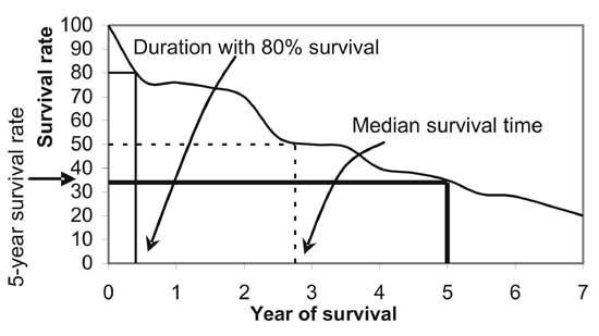
Plot of survival function against the end-point of the time interval, when joined by lines, is the survival curve. Although software will give you the estimated median survival time, you can also obtain approximate value of median by drawing horizontal line at 50% survival rate and reading the corresponding survival time on the x-axis. The survival curve can also be used to estimate other parameters of interest such as 5-year survival rate, or the duration when 80% of the subjects survive. All these are illustrated in Fig 2.

Fig. 2 Using survival curve for obtaining various estimates.

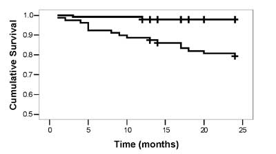
Statistical software will require that the censored values are identified by a particular (software dependent) value, for instance 0 for censored cases and 1 for fully known durations. The software will estimate the (cumulative) survival probability at every time point based on censored and complete values, and will plot the survival curve of the type shown in Fig 3. Survival curve for samples is a piecewise function where straight lines with constant slope are connected at the ends of intervals.

Fig. 3 Survival curves in two groups under comparison (censored values are shown by + sign).

Kaplan-Meier (K-M) method of survival analysis is used when the subjects are continuously observed and exact duration of reaching to the end-point or at the time of dropout is known. Dropouts are considered in the analysis till the time they dropped out and after that they are ignored since they are no longer considered at risk for the end-point. Intuitively this looks most sensible thing to do for censored values to avoid bias. Censored subjects should follow the same survival pattern as those available.

Proportions survived of those at risk are obtained for each unique time point at which an event occurred and the estimated survival function (proportion surviving since the beginning) is obtained again by sequential multiplication as for life-table method.

Kaplan-Meier method gives more accurate results than life-table method. Interval censoring amounts to loss of some information that affects the efficiency of the estimates. Thus, prefer continuous observation of survival process so that exact time of survival or of dropout is known for each subject unless n is really large and periodic observations are cost-effective.

Plot of survival function against time is the survival curve and can be used to estimate median survival time, quantiles and other measures of the survival distribution. In this case, the survival curve is a step function which moves down whenever deaths occur.

The two methods discussed so far are for obtaining the survival function that estimates survival probability for different time points. Now consider the problem of comparing survival pattern in one group with another such as in males and females, or in treatment and control groups. If each time point has the same importance as another, log-rank test is often used to compare the survival curves. In rare cases, some investigators may be interested in giving more weight to the time point where more number of subjects is available. Then log-rank is not appropriate. Other methods such as generalized Wilcoxon rank-sum test are used in this case(9). This method is also known as Gehan and Breslow test. Since weighted by the number of subjects at risk, this method gives higher weight to initial time points.

Log-rank method works on the same principle as Kaplan-Meier and thus requires that survival duration is exactly available for both groups. Expected deaths at each time point in either group are obtained by following a procedure similar to the one followed for the contingency tables. Total expected deaths for group-I and group-II are compared with the total observed deaths in group-I and group-II, respectively, and a chi-square value with 1 degree of freedom is obtained. This is used to reject or not reject the null hypothesis of equality of survival curves. For details of calculations, see Indrayan(10). Log-rank method does not work for interval-censored data. Kim, et al.(11) has proposed a variation of log-rank that may be applicable to interval-censored data.

The log-rank test gives valid and easily interpretable results when one survival curve is consistently higher than the other (Fig 3). This figure is for the data on different antibody levels (Group I – where peak antibody level is below 15% and Group II – where it exceeds 15%) in patients of renal allograft. The dataset in MSExcel is available at http://www.medicalbiostatistics.com for those who want to try. If they cross so that survival in one group is better up to a particular time point, say 3 years, and worse thereafter, the log-rank method loose validity.

A step further in survival analysis is to be able to delineate the role of factors called covariates that affect duration of survival. This is commonly done by Cox model. The covariates can be continuous or categorical.

A basic requirement of Cox model is proportional hazard. Hazard considers failure instead of survival. In a severe earthquake, the hazard of death per hour in affected area is extremely high relative to hazard of death in motor vehicle accidents.

Hazard naturally changes when one or more risk factors are present. Hazard of discontinuing breastfeed steeply increases with every passing month in working women relative to women at home. Theory of relativity works in full measure here and hazard ratio is studied instead of hazard alone. Hazard in women at home can be considered baseline and hazard ratio in working women may be 3.1 at 3 months and 4.5 at 6 months. 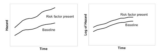This ratio could be different at different time points. Cox model requires that the hazard ratio must remain same over the entire duration under consideration, i.e., if hazard increases by 10% every month, this should be so for working women as well as for women at home in our example. Mathematically this means that logarithm of hazards are parallel (Fig 4). This condition is popularly called proportional hazards. A figure of the type in Fig 4 helps in case of one covariate but not for multiple covariates. But the figure explains the underlying requirement very well. The figure does not assess the statistical significance of deviation from parallelism. One method to check this is to test for interaction of log-time with each covariate by a test such as Wald’s test. Check if your software has this provision. Graphical plot should be adequate in most cases.

Fig. 4 Graphs showing meaning of proportional hazards.

In Cox model, the logarithm of hazard ratio is modeled relative to a baseline as a linear function of covariates. The cumulative survival function can be obtained from the cumulative hazard function through a simple mathematical relation(12). The censored values are adequately accounted for and contribute substantially to the model building process.

Consider duration of survival of peritonitis cases after surgery. This can be modeled to depend on the severity of disease at the time of admission measured by APACHE score, age of the patient and sex of the patient, beside other relevant factors. You can estimate the effect of APACHE score on the duration of survival or test a hypothesis regarding sex differentials in survival pattern. If the number of subjects in any subgroup is extremely small or zero, you can get weird results such as extremely large coefficients or large standard error. This can also happen when covariates are strongly related, called multicolinearity. This underscores the need to carefully scrutinize the data for suitability of Cox model. The bottom line is the investigator himself who has to take all the responsibility.

Risk factors in Cox model can be continuous such as birth weight in breastfeeding example or categorical such as working status of the woman. An important requirement of the usual Cox model is that these risk factors should be time invariant. They should not change during the period of the study. Whereas birth weight in this example fulfills this criterion as it is a measurement before the onset of study but working status may change during the six month period if that is the period of the study. Age of the patient at onset of a disease is time invariant but age during long follow-up is not. If the covariates are time dependent, Cox model is still applicable but the method becomes complex(13). Nonetheless, computer will go through its gyrations and come up with an answer. This may leave an unenviable task for you to interpret the coefficients since caution is required.

For further details of various survival methods and related intricacies, see reference 9.

Contributors: AI: prepared the initial manuscript and provided technical inputs. AKB: collected all the supporting material and completed the manuscript. Both reviewed the final manuscript.

Funding: None.

Competing interests: None stated.

1. Hirve S, Ganatra B. A prospective cohort study on the survival experience of under five children in rural western India. Indian Pediatr 1997; 34: 995-1001.

2. Lee SJ, Ahn SJ, Lee JW, Kim SH, Kim TW. Survival analysis of orthodontic mini-implants. Am J Orthod Dentofacial Orthop 2010; 137: 194-199.

3. Giashuddin MS, Kabir M. Breastfeeding duration in Bangladesh and factors associated with it. Indian J Comm Med 2003; 28: 34-38.

4. Schaefer F, Marr J, Seidel C, Tilgen W, Scharer K. Assessment of gonadal maturation by evaluation of spermaturia. Arch Dis Child 1990; 65: 1205-1207.

5. Bajpai A, Kabra M, Gupta AK, Menon PSN. Growth pattern and skeletal maturation following growth hormone therapy in growth hormone deficiency: factors influencing outcome. Indian Pediatr 2006; 43: 593-599.

6. Sarin M, Dutta S, Narang A. Randomized controlled trial of compact fluorescent lamp versus standard phototherapy for the treatment of neonatal hyperbilirubinemia. Indian Pediatr 2006; 43: 583-590.

7. May M, Sterne J, Egger M. Parametric survival models may be more accurate than Kaplan-Meier estimates. BMJ 2003; 326: 822.

8. Utley M, Gallivan S, Young A, Cox N, Davies P, Dixey J, et al. Potential bias in Kaplan-Meier survival analysis applied to rheumatology drug studies. Rheumatology (Oxford) 2000; 39: 1-2.

9. Hosmer DW, Lemeshow S. Applied Survival Analysis: Regression Modeling of Time to Event Data. Wiley New York: Interscience; 1998.

10. Indrayan A. Survival Analysis. In: Medical Biostatistics. IInd ed. New York: Chapman & Hall/CRC Press; 2008: pp. 620-622.

11. Kim J, Kang DR, Nam CM. Logrank-type tests for comparing survival curves with interval-censored data. Comput Stat Data Analys 2006; 50: 3165-3178.

12. Bewick V, Cheek L, Ball J. Statistics review 12: Survival analysis. Crit Care 2004; 8: 389-394.